Generate filtering column (Excel Options)
The
Generate filtering column option
of Excel Options
allows you to filter the rows for display on your Excel report.
A
hidden column is added to the Excel report. If you are using Cell
Borders, the hidden column is Column B, if you are not using Cell
Borders, the hidden column is Column A.
The
example below is using Cell Borders
so Column B is the hidden column:
- Open the Excel report and highlight
Columns A and C.
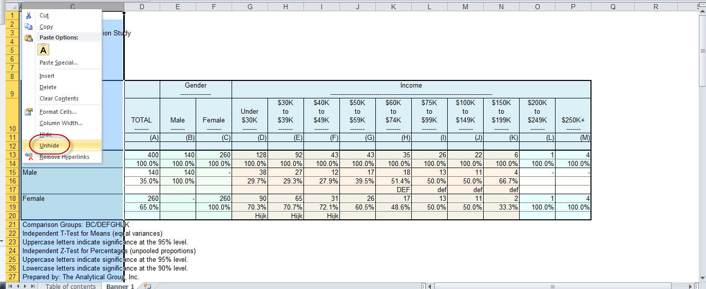
- Right-click and select Unhide
to display the contents of Column B.
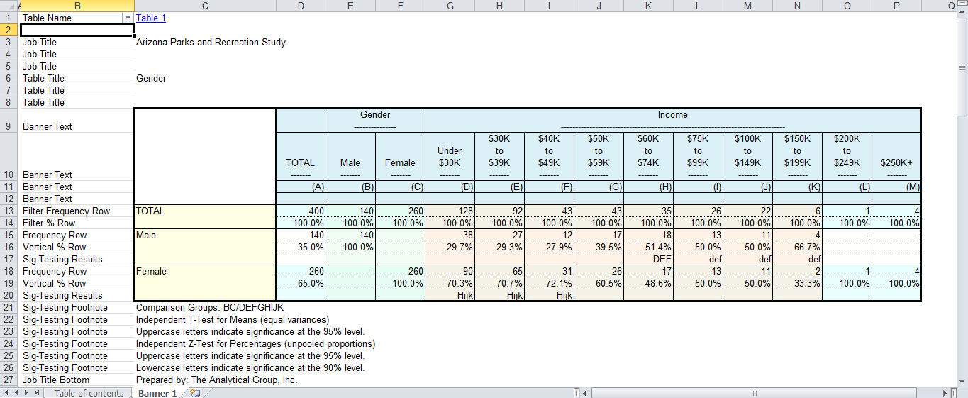
- Notice that each row of the Excel
file has a WinCross row type in Column B (for example, Banner
Text, Filter Frequency Row,
Filter % Row, etc.).
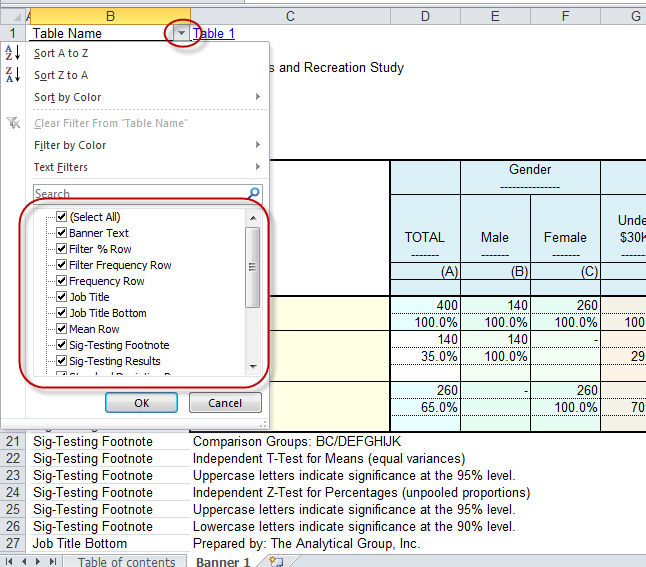
- Select the dropdown arrow in the
upper right-corner of Column B to display the filtering display options.
- Select
All is the WinCross default for the filtering display options.
- Choose the rows that you want to
show or hide by clicking the check box next to each row type.
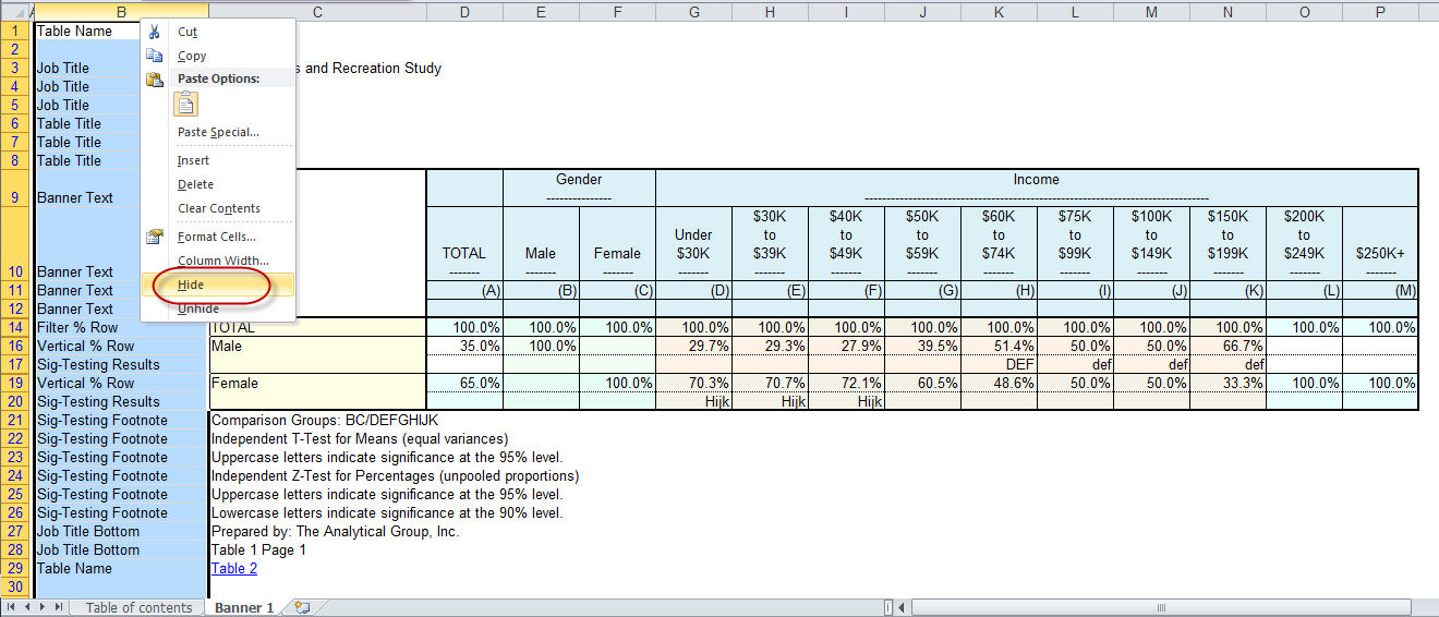
- Highlight Column B, right-click and
choose Hide to re-hide Column
B after making your filtering choices.
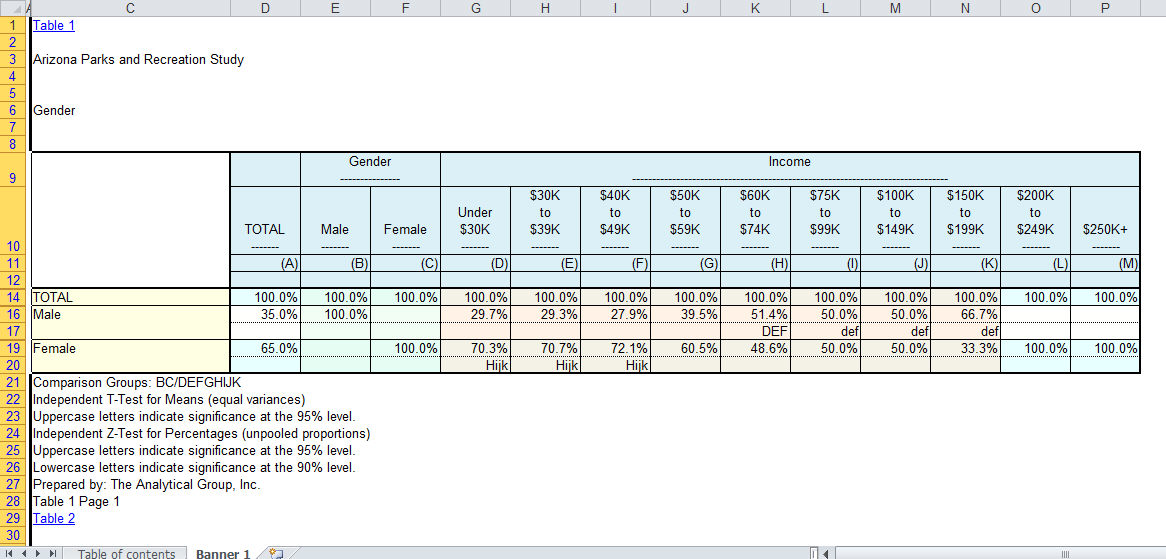
- In this example, we unchecked the
Filter Frequency Row and Frequency Row check boxes and are
showing a table with percents and significance testing and no frequencies.
Filtering
Considerations:
- When using the Worksheet
options of Create each table
as a separate worksheet, one banner per workbook or Create
each table as a separate worksheet, all in one workbook, the
filtering options will need to be applied to each table (worksheet).
There is no way to set the filtering options for all tables at once
when each table is a separate worksheet.
- When using the Worksheet
option of Create one banner
per worksheet, all in one workbook, the filtering options will
need to be applied to each banner (worksheet).
- When the Formatting
options of Below, in a separate
cell, To the right, in the
same cell or To the right,
in a separate cell are used, the significance indicator will
be written with the Frequency Row
and cannot be hidden separately from the Frequency.
Use the Below, in a separate cell
option if you want to show or hide the Sig-Testing
Results differently than the Frequency
Row.
Related topics:
Excel Options